
“What gauge do I need?” is really three questions bundled together: how much voltage drop can the load tolerate, how much current must the conductor carry, and what temperature can the insulation survive. Most catalog tables only answer the second one. On a 24 V machine circuit that is the wrong order — one volt of loss is 4.2 % of the supply, so length, not current, is usually what forces the bigger conductor.
This guide gives you the arithmetic, the conductor data and the failure points to answer all three. Everything below is indicative engineering data derived from published conductor standards and the resistivity of plain copper; confirm the final construction against the applicable standard and the cable maker’s data sheet for your exact stranding and insulation.
1. On low-voltage DC, voltage drop decides — not ampacity
The same 1 V of voltage drop costs you very different things depending on system voltage:
| Nominal system voltage | 1 V of drop is | Volts available at a 3 % limit | Volts available at a 5 % limit |
|---|---|---|---|
| 5 V (USB rail) | 20 % | 0.15 V | 0.25 V |
| 12 V | 8.3 % | 0.36 V | 0.60 V |
| 24 V | 4.2 % | 0.72 V | 1.20 V |
| 48 V | 2.1 % | 1.44 V | 2.40 V |
| 110 V DC | 0.9 % | 3.30 V | 5.50 V |
| 230 V AC | 0.43 % | 6.90 V | 11.50 V |
Industrial DC control and power circuits typically work to a 3–5 % budget; some loads (solenoid valve islands, sensors near their low-voltage threshold, DC-DC charger inputs) are tighter still. The limit comes from the load’s own tolerance, not from a single universal number.
A 3 A load on an 18 AWG (0.82 mm²) flexible cable sits well inside any ampacity table — 6.6 A per core in a four-core bundle. Yet push the same 3 A through 5 m of it at 24 V and the copper alone consumes 3.5 % of the supply: 2.6 % on plain copper at 20 °C, 3.5 % once the stranding and conductor-temperature corrections of §3 and §4 are applied. Against a 3 % budget, that cable is already out of spec at a length shorter than most machine looms. The conductor was never the problem; the run was. That is why the first calculation is a resistance budget, not a current check.
The resistance budget — rearrange the voltage drop equation once, then shop for a gauge
Instead of guessing a gauge and testing it, solve the drop limit for the maximum conductor resistance you can afford. Take the one equation of §2, V = 2 L I ρ / A, and rearrange it for the resistance term ρ / A:
Worked: 24 V system, 3 % allowed, 3 A, one-way length 2 m.
(3 × 24) / (100 × 2 × 3 × 0.002) = 60 Ω/kmper conductor to spend.
You are now shopping, not calculating. Any conductor whose one-way resistance at its service temperature is 60 Ω/km or less will pass — §7 does exactly that. The same move works for any voltage, current or length, which is why it is the most reusable trick in cable sizing: solar strings, valve islands, machine interlocks, 48 V power feeds, USB charging leads. The answer is per conductor; if the source you are comparing against quotes the loss for the whole loop, it will read about twice this value.
2. The voltage drop equation, and the four values it needs
For a two-wire circuit the voltage drop is a straight application of Ohm’s law to the resistance of the copper in the path. This is the only equation used in this article:
| Symbol | Meaning | Units we use |
|---|---|---|
| Vdrop | Volts lost between the source terminals and the load terminals | V |
| L | One-way length of the run, source to load | m |
| I | Design current — the highest sustained current, not the average | A |
| ρ | Resistivity of the conductor material. Plain copper at 20 °C: 1.724 × 10⁻⁸ Ω·m | Ω·m |
| A | Conductor cross-sectional area in square metres — so 1.5 mm² enters as 1.5 × 10⁻⁶ m² | m² |
Unit traps: L must be one-way, and A must be converted from mm² to m². Both are simple, and both are the origin of most order-of-magnitude errors.
Why the 2 is there
Current leaves the source on one conductor and must come back on another, so the loop contains two lengths of copper. The 2 accounts for the return path, and it is the reason a 2 m cable behaves like 4 m of conductor.
The multiplier changes with circuit topology:
| Circuit | Multiplier on the conductor term |
|---|---|
| Two-wire DC (supply and separate return) | 2 |
| Single-phase AC | 2 (resistance only; add reactance on large sizes or long runs) |
| Balanced three-phase | √3 ≈ 1.732 for the line-to-line voltage drop |
| Return through the machine frame or a bonded structure | 1 — the frame is the return, but add the resistance of every bolted joint and watch for galvanic corrosion at those interfaces |
3. Stranding: why the same mm² can be 16 % more resistive
ρ / A describes a solid, geometrically perfect conductor of exactly the nominal area. A real conductor is a helix of many strands, each of which is longer than the cable axis, and the actual copper area differs from nominal within a permitted tolerance. The practical result is that the ideal formula understates resistance by a margin that depends on the stranding class you choose. Call that margin kS — the stranding factor, applied as a multiplier on resistance.
| Nominal area | Ideal ρ/A (Ω/km) | Class 2 actual, max (Ω/km) | kS | Flexible Class 5/6 actual, max (Ω/km) | kS |
|---|---|---|---|---|---|
| 0.5 mm² | 34.5 | 36.0 | 1.04 | 39.0 | 1.13 |
| 0.75 mm² | 23.0 | 24.5 | 1.07 | 26.0 | 1.13 |
| 1.0 mm² | 17.2 | 18.1 | 1.05 | 19.5 | 1.13 |
| 1.5 mm² | 11.5 | 12.1 | 1.05 | 13.3 | 1.16 |
| 2.5 mm² | 6.90 | 7.41 | 1.07 | 7.98 | 1.16 |
| 4 mm² | 4.31 | 4.61 | 1.07 | 4.95 | 1.15 |
| 6 mm² | 2.87 | 3.08 | 1.07 | 3.30 | 1.15 |
| 10 mm² | 1.72 | 1.83 | 1.06 | 1.91 | 1.11 |
| 16 mm² | 1.08 | 1.15 | 1.07 | 1.21 | 1.12 |
| 25 mm² | 0.69 | 0.727 | 1.05 | 0.780 | 1.13 |
Indicative maxima at 20 °C for plain annealed copper, per IEC 60228 conductor classes. Class 6 (extra-flexible) resistance limits are close to Class 5; in practice finer stranding with shorter lays can measure slightly higher. Always use the maker’s value for the exact construction.
Two conclusions that change designs:
- Fixed stranded (Class 2): kS ≈ 1.05. Small enough to absorb in a margin — but not if your budget had no margin.
- Flexible (Class 5/6): kS ≈ 1.13. Choosing a flexible cable for a drag chain, a robot axis or a handheld tool is not free: you pay roughly 13 % more resistance for the same nominal area. If you sized the gauge with the bare ideal value, you have silently spent part of a gauge. This is the commonest reason a “correctly calculated” flexible assembly measures a higher voltage drop than predicted.
4. Temperature: the second correction
Published resistances are almost always stated at 20 °C, and a loaded conductor never stays there. Copper resistance rises with temperature:
Write the bracket as kT, the temperature factor, and it multiplies straight onto the resistance in the same equation.
| Conductor temperature | kT | Typical conductor that lives here |
|---|---|---|
| 20 °C | 1.000 | Reference temperature of most tables |
| 40 °C | 1.079 | Lightly loaded control wiring |
| 60 °C | 1.157 | Loaded PVC wiring in a warm cabinet |
| 70 °C | 1.197 | PVC at its rating; the basis of standard thermoplastic voltage-drop tables |
| 80 °C | 1.236 | PUR / TPU at its rating |
| 90 °C | 1.275 | XLPE / TPE at their rating |
| 105 °C | 1.334 | 105 °C PVC, some XLPE |
| 125 °C | 1.413 | High-temperature TPE and cross-linked compounds |
Design at the conductor’s maximum rated temperature, not at 20 °C. A 2.5 mm² flexible conductor moves from 7.98 Ω/km at 20 °C to about 9.55 Ω/km at 70 °C — a 20 % change, which is larger than most design margins. At 90 °C the same conductor is up about 27 %.
One more consequence: the hottest point governs the whole run. Where a cable crosses a hot zone and then ages out in ambient air, both the insulation rating and the resistance take their worst case from that hot section — a short hot segment can invalidate an otherwise comfortable calculation.
5. Ampacity is the second check, not the first
Ampacity answers a different question: how hot will the conductor get, and can the insulation survive it? Published tables come in two families that answer slightly different questions, and mixing them up is the reason two engineers can disagree by a factor of three:
- Conservative (density and voltage drop) values — roughly 700 circular mils per amp. These are the right basis for real runs, because they implicitly respect both heat and drop.
- Thermal values for a single conductor in free air — roughly 200 circular mils per amp, so three to four times higher. These describe one conductor alone, still air, no enclosure, no neighbours.
| AWG | mm² | Conservative basis (A) | Single conductor, free air (A) | 4–6 core jacketed bundle, ~0.7 derate (A) |
|---|---|---|---|---|
| 28 | 0.081 | 0.23 | 0.83 | ≈ 0.6 |
| 26 | 0.129 | 0.36 | 1.3 | ≈ 0.9 |
| 24 | 0.205 | 0.58 | 2.1 | ≈ 1.5 |
| 22 | 0.324 | 0.92 | 3.5 | ≈ 2.5 |
| 20 | 0.519 | 1.5 | 5.6 | ≈ 3.9 |
| 18 | 0.823 | 2.3 | 9.5 | ≈ 6.6 |
| 16 | 1.31 | 3.7 | 15 | ≈ 10 |
| 14 | 2.08 | 5.9 | 24 | ≈ 17 |
| 12 | 3.31 | 9.3 | 37 | ≈ 26 |
| 10 | 5.26 | 15 | 58 | ≈ 41 |
Indicative per-conductor values at about 30 °C ambient, PVC-insulated. The bundle column applies roughly 0.7 to the free-air column to account for neighbours and a jacket that blocks convection; a genuinely tight or potted construction is worse still.
Apply the derating factors before you trust any of it:
- Bundling — more than three current-carrying conductors in a bundle, jacket or conduit trap heat. Common practice is about 0.8 for four to six conductors, 0.7 for seven to nine, and 0.5–0.6 beyond that. A shielded multicore is a closed heat path by construction.
- Ambient temperature — a 105 °C-rated cable in a 60 °C cabinet has far less headroom than the same cable in a 25 °C room.
- Enclosure — free air, sealed panel, potted overmold and buried conduit all dissipate heat differently. An overmolded body is thermally closed by design.
- Duty cycle — continuous versus intermittent changes the steady-state rise.
Multi-core cables: count every conductor that carries current
A single conductor’s ampacity is not the cable’s ampacity. Three counting rules cover most of the mistakes:
- Both conductors of a two-wire circuit carry the full current. A 2-conductor power pair therefore dissipates
2 I²Rper metre, and the loop voltage drop carries the same factor 2 that stands in front of the equation in §2. Two conductors means twice the heat inside one jacket. - Signal pairs that carry no power current do not count toward the bundle load — but the jacket still has to shed the heat from the conductors that do. A two-power-core plus one-data-pair construction is thermally a bundle, not a single wire.
- Never use a screen or drain wire as a return. A drain conductor is sized for screening, typically 28–30 AWG equivalent, and its resistance per metre is far too high to carry load current; it will also radiate the noise you were screening against.
So a “4-core” cable does not give you four times the current of one core. In a jacketed, shielded four-conductor construction, work from the bundle column above — and if the cable runs warm or sits in a cabinet, take the next size up.
Worked check: a 24 AWG × 2C power pair at 2 A, 3 A and 5 A
A very common construction is 24 AWG × 2C for power, 28 AWG × 1P for data, plus a drain and a shield. Both power conductors carry the full load current, so this is a two-wire circuit inside a four-conductor bundle. Take the numbers in three steps.
Step 1 — resistance of the power conductor. 24 AWG is 0.205 mm². The ideal one-way resistance is 84 Ω/km; with a stranding factor of about 1.07 for a fine-strand power core, call it 90 Ω/km at 20 °C. At a 70 °C conductor temperature, kT = 1.197 gives about 108 Ω/km.
Step 2 — voltage drop over a 1 m cable. Using the equation of §2 with the resistance above:
| Load current | Loop resistance at 20 °C (2 × 90 Ω/km × 1 m) | Vdrop at 20 °C | Vdrop at 70 °C |
|---|---|---|---|
| 2 A | 0.180 Ω | 0.36 V | 0.43 V |
| 3 A | 0.180 Ω | 0.54 V | 0.65 V |
| 5 A | 0.180 Ω | 0.90 V | 1.08 V |
Those volts look small until you express them as a percentage of what is being delivered — which is exactly the mistake people make when they judge a 5 V charging cable:
| Supply voltage | 0.43 V @ 2 A | 0.65 V @ 3 A | 1.08 V @ 5 A | Verdict |
|---|---|---|---|---|
| 5 V (USB 2.0 / BC 1.2 charging) | 8.6 % | 13.0 % | 21.6 % | Fails — the device sees well under 4.75 V |
| 9 V (USB PD) | 4.8 % | 7.2 % | 12.0 % | Marginal at 2 A, fails above |
| 12 V | 3.6 % | 5.4 % | 9.0 % | Acceptable at 2 A only |
| 20 V (USB PD 3.0) | 2.2 % | 3.3 % | 5.4 % | Acceptable to 3 A |
| 48 V (USB PD 3.1 EPR) | 0.9 % | 1.4 % | 2.3 % | Comfortable |
This one table explains a phenomenon most people meet before they meet the theory: the same 24 AWG cable that charges a laptop perfectly at 20 V is hopeless at 5 V. Nothing about the cable changed. Voltage drop is a fixed number of volts, and its significance is set by the system voltage. The Power Delivery case — where the USB-IF test specification sets its own cable IR-drop budget instead of a percentage — is worked through in USB PD cable gauge.
Step 3 — the honest length limit at 5 V. Taking a 5 % budget (0.25 V) and solving for length:
- At 2 A:
L = 0.25 / (2 × 2 × 0.09) = 0.69 m - At 3 A:
L = 0.25 / (2 × 3 × 0.09) = 0.46 m - At 5 A:
L = 0.25 / (2 × 5 × 0.09) = 0.28 m— and the thermal limit rules this out long before voltage drop does.
Thermally, the same cable is also working hard. At 2 A each power conductor dissipates I²R = 4 × 0.09 = 0.36 W per metre, so the pair sheds about 0.72 W/m; at 3 A that becomes roughly 1.6 W/m on a cold basis and more once hot; at 5 A it is about 4.5 W/m. Against a bundled limit near 1.5 A per conductor for 24 AWG, 2 A is already slightly over, 3 A is roughly double, and 5 A is a connector-melting condition. Expect a cable that is noticeably warm, and connectors warmer still — the contact resistance inside a molded connector is usually the real hot spot, even though its contribution to voltage drop at these currents is small.
- 2 A — borderline, acceptable only as a short lead. Keep it under about 0.5 m at 5 V, keep the ambient sensible, and do not bundle it with other loaded cables. Thermally it sits right at the limit of a jacketed bundle.
- 3 A — not acceptable on 24 AWG. Move the power pair to 20 AWG (0.519 mm²), which takes the one-way resistance from 90 Ω/km to about 36 Ω/km at 20 °C and brings a 1 m cable back to roughly 0.21–0.26 V, i.e. 4–5 % at 5 V. For genuine margin at 3 A and 5 V, specify 18 AWG (0.823 mm²) for the power pair — about 22 Ω/km, roughly 0.16 V, 3.2 %.
- 5 A — unsafe on 24 AWG. About 4.5 W/m in the pair against a bundled limit of 1.5 A per conductor: this is the failure mode that ends in a hot or discoloured connector shell. The power pair must be 18 AWG minimum for 5 A in a jacketed construction.
- At 20 V and above the same 24 AWG pair is fine on voltage drop grounds, which is why the construction is legitimate in Power Delivery cables and not in 5 V charging leads.
- The 28 AWG pair, the drain and the shield carry no power current and must not be reused as a return path.
For a USB-style or multi-function cable the practical sequence is: fix the system voltage first, then the current, then let the voltage drop budget pick the power-pair gauge, and only then check the bundle thermally. Doing it in the opposite order is how a cable ends up technically “rated” but unusable in service.
6. Insulation temperature rating sets the ceiling
| Insulation / jacket | Typical continuous rating | Practical note |
|---|---|---|
| PVC | 70 °C (105 °C special grades) | Lowest cost; softens and ages with heat; standard flexible-jacket material |
| PE | 70–80 °C | Good dielectric for fixed data runs |
| XLPE | 90 °C (125 °C for some) | Strong dielectric, moderate flex |
| TPE | 90–125 °C | Flexible, halogen-free options, good cold flexibility |
| PUR / TPU | 80–90 °C | Best oil, abrasion and cut resistance; lower heat ceiling |
| Silicone | 180–200 °C | Very high heat and cold flexibility; lower mechanical strength |
| FEP / PFA | 200–260 °C | High heat plus chemical resistance, at a cost |
Indicative ratings for the compound families; confirm the actual grade with the maker.
The rating is a double constraint. It caps ampacity and it sets the temperature at which you must evaluate resistance — a 105 °C PVC grade lets you carry more current, but §4 says you must then calculate the drop at a conductor about 33 % more resistive than at 20 °C. Choosing a high-temperature compound to win the ampacity check can lose you the voltage-drop check on the same run.
7. A complete selection, using the same equation
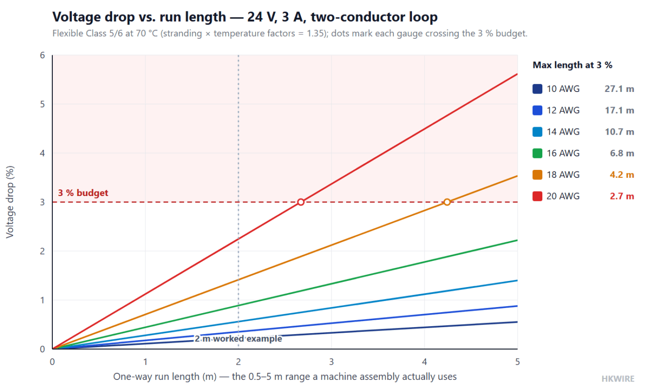
Scenario: a 24 V DC valve island drawing 3 A at the end of a 2 m one-way run, in a flexible assembly, with a 3 % voltage drop budget (0.72 V).
Step 1 — spend the budget. From §1: (3 × 24) / (100 × 2 × 3 × 0.002) = 60 Ω/km per conductor allowed.
Step 2 — compare gauges. The uncorrected column applies V = 2 L I ρ / A to plain copper at 20 °C. The design column applies the two corrections from §3 and §4: kS = 1.13 for flexible Class 5/6 stranding and kT = 1.197 for a 70 °C conductor — a combined factor of 1.35 on resistance.
| Gauge | One-way R, ideal (Ω/km) | Vdrop uncorrected | % of 24 V | One-way R at 70 °C (Ω/km) | Vdrop, corrected | % of 24 V |
|---|---|---|---|---|---|---|
| 24 AWG (0.21 mm²) | 84.1 | 1.01 V | 4.2 % — fail | 113.5 | 1.36 V | 5.7 % — fail |
| 22 AWG (0.32 mm²) | 53.2 | 0.64 V | 2.7 % — marginal pass | 71.8 | 0.86 V | 3.6 % — fail |
| 20 AWG (0.52 mm²) | 33.3 | 0.40 V | 1.7 % — pass | 44.9 | 0.54 V | 2.2 % — pass |
| 18 AWG (0.82 mm²) | 21.0 | 0.25 V | 1.0 % — pass | 28.3 | 0.34 V | 1.4 % — pass |
Read the two rows for 22 AWG together. Uncorrected, 22 AWG looks acceptable at 2.7 %; corrected for flexible stranding at a 70 °C conductor, it fails at 3.6 %. The corrections are not exotic margin-padding — they are the difference between a prediction and what the installed cable will actually measure:
- Flexible stranding instead of ideal solid copper: +13 % (from §3).
- 70 °C instead of 20 °C: +20 % (from §4).
- Combined: ≈ +35 % on resistance — comfortably more than a full gauge.
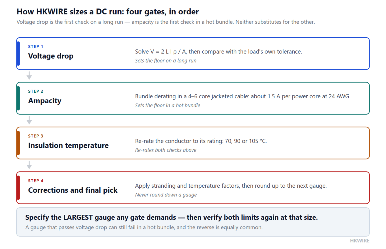
So for this run we would quote 20 AWG (0.52 mm²), IEC 60228 Class 5/6 tinned or plain copper, PVC 70 °C or better — inside the voltage drop budget with margin, and inside the 3.9 A bundle ampacity of §5 with about 30 % headroom. And when a customer asks why their own calculation said 22 AWG, the answer is the stranding factor and the conductor temperature, not a disagreement about arithmetic.
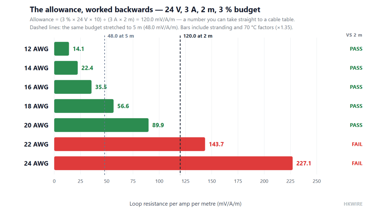
Both gates land on the same size here, which is worth pausing on because it is not the usual outcome. The drop check allowed 60 Ω/km and the 20 AWG conductor presents 44.9 Ω/km at 70 °C, so it clears with room; the bundle ampacity of §5 gives 20 AWG about 3.9 A against a 3 A load. Move the same valve island out to 5 m and the drop check takes over and pushes the answer to 16 AWG. Bring it in to 0.5 m and the drop check would allow 26 AWG, at which point ampacity and handling — not voltage drop — decide the gauge. Length decides which gate leads.
| One-way run | Allowance per conductor | Loop allowance (mV/A/m) | Thinnest gauge the drop check allows |
|---|---|---|---|
| 0.5 m | 240 Ω/km | 480 | 26 AWG |
| 1 m | 120 Ω/km | 240 | 24 AWG |
| 2 m | 60 Ω/km | 120 | 20 AWG |
| 3 m | 40 Ω/km | 80 | 18 AWG |
| 5 m | 24 Ω/km | 48 | 16 AWG |
Same 24 V, 3 A and 3 % budget throughout — only the length changes. Machine assemblies rarely run past about 5 m, so this is the whole range that matters in practice, and the allowance moves by a factor of ten across it. Loop figures and gauge comparisons use flexible Class 5/6 at 70 °C (×1.35 on resistance); below about 2 m the 3.9 A bundle ampacity of §5 becomes the binding limit rather than voltage drop.
Connection resistance: the milliohm budget
The equation covers copper. It does not cover the crimp, the terminal, the contact or the fuse. Those are negligible at low current and dominant at high current:
| Circuit current | Voltage drop across a 10 mΩ connection pair | Effect on a 24 V system |
|---|---|---|
| 3 A | 0.03 V | 0.13 % — negligible |
| 20 A | 0.20 V | 0.83 % — worth counting |
| 100 A | 1.00 V | 4.2 % — larger than most cable allowances |
Above roughly 50 A, high-current DC assemblies should be specified by a milliohm budget for the whole path — conductor, crimp, contact, fuse — rather than by gauge alone. Contact resistance is also the part that degrades: it creeps up with corrosion, fretting and thermal cycling, which is why an installation can pass on day one and fail a year later without anything being touched.
Verifying a run on site
- Measure under rated load, not open circuit. A no-load reading proves continuity, not voltage drop.
- Measure across the load terminals, with the meter’s leads on the two points the load actually sees — that captures the whole loop including connections.
- Use a four-wire (Kelvin) method for expected drops below a few hundred millivolts; two-wire lead resistance can be a meaningful fraction of the reading.
- Log the current at the same time, then compare the reading with the prediction at that current.
- Read the diagnostic signature. Voltage drop that scales linearly with current is a conductor-gauge or length issue. Voltage drop that is far higher than a linear prediction, or that jumps between readings, points at a joint. Voltage drop that grows over months with no change in load indicates corrosion or loosening at a termination.
For a charging cable the same method reduces to one number: drive the rated current through the cable, read the voltage across the two ends, divide by the current, and halve it if you want the one-way value. That figure — milliohms per metre, or millivolts per amp per metre — is the only charging-cable specification a buyer cannot be misled about.
What to put on the drawing
- Nominal area in mm² and the AWG equivalent.
- Stranding class to IEC 60228 (Class 2 fixed, Class 5/6 flexible) — this is what makes the resistance reproducible.
- Conductor material and plating requirement.
- Maximum conductor temperature and the insulation rating that allows it.
- Allowable voltage drop with the current and temperature at which it applies.
- Length basis stated explicitly as one-way or loop.
- For a PD cable, the current capability (3 A or 5 A), the e-marker requirement and the speed class of the data pairs.
- The test method to be used for acceptance (loaded, four-wire, at terminals).
Conductor selection feeds directly into the rest of the assembly: see the DC power cable range for pre-terminated power runs, custom wire harnesses for multi-conductor looms built to a drawing, and custom development when the connector itself has to be molded around the cable.
Frequently asked questions
Do I use the one-way length or the whole loop?
Put the one-way length into the equation; the factor 2 already accounts for the return conductor. If the table or drawing you are working from quotes a loop length, halve it before you start. Stating the length basis is the single most effective way to stop two engineers disagreeing about a voltage-drop number.
Why does my flexible cable measure a higher voltage drop than calculated?
Two corrections stack. Flexible Class 5/6 stranding carries roughly 11–16 % more resistance than the ideal ρ/A value for the same nominal area, and a loaded conductor operates well above 20 °C, adding about 20 % at 70 °C and 27 % at 90 °C. Together that is roughly 35 % — usually more than a full gauge.
Can I use a resistance table stated at 20 °C?
Only if you also intend the conductor to run at 20 °C, which a loaded conductor does not. Multiply by kT = 1 + 0.00393 (T − 20) at the maximum rated temperature of the insulation, or use a table already published at that temperature.
How much current can one core of a multi-core cable carry?
Less than the same gauge in free air. Start from the single-conductor value, then apply a bundle derating factor — about 0.8 for four to six current-carrying conductors, 0.7 for seven to nine, 0.5–0.6 above that, and worse for a tight or potted jacket. For 24 AWG that means roughly 1.5 A per conductor in a jacketed four-core construction, not the 2.1 A free-air figure.
Is a 24 AWG × 2C power pair safe at 2 A or 3 A?
At 2 A it is borderline: slightly over the bundled thermal limit and outside a 5 V drop budget beyond about 0.5–0.7 m. At 3 A it is not acceptable — move the power pair to 20 AWG, or 18 AWG if you want genuine margin at 5 V. At 5 A it is unsafe in a jacketed construction: 18 AWG minimum. At 20 V and above the same 24 AWG pair is fine on drop grounds, which is why the construction is common in Power Delivery cables but not in 5 V charging leads.
Does aluminum or copper-clad aluminum change the answer?
Yes. Aluminum resistivity is about 2.826 × 10⁻⁸ Ω·m, roughly 64 % above copper, so the same gauge drops about 1.6 times as much. Copper-clad aluminum sits between the two and carries considerably less current than solid copper of the same diameter. Verify the conductor material before designing around a price.
What is the multiplier on a three-phase circuit?
Not 2. A balanced three-phase circuit uses √3 (≈ 1.732) for the line-to-line drop. If the return path is the machine frame or a bonded structure, the conductor is counted once — but add the resistance of the bolted joints and watch for galvanic corrosion at those interfaces.